Introduction to Process Performance Qualification (PPQ) Sampling Plan R Package
Yalin Zhu (yalin.zhu@merck.com)
2021-11-02
Source:vignettes/PPQplan-vignette.Rmd
PPQplan-vignette.RmdThis vignette summarizes the functions in the PPQplan package, and provides some examples to illustrates how to use the package.
Note: in order to better perform the dynamic plots, it is recommended to run the following code in RStudio.
devtools::load_all()## ℹ Loading PPQplanFunctions
This package provides several S3 functions listed as follows:
rl_pp: calculates probability of pass the specification test.
Example: Consider some sterile concentration assay as a CQA, the lower and upper specification limits are 95% and 105%, if the hypothetical mean and standard deviation are 98% and 1%, then the probability of passing the specification test will be calculated as follow.
rl_pp(Llim=95, Ulim=105, mu=98, sigma=1)## [1] 0.9986501The following four functions are mainly for the sampling plan using statistical intervals with general multiplier
PPQ_ppPPQ_occurvePPQ_ctplotPPQ_ggplot
For the above example, assume the PPQ study reports a sample of 10 assay results per batch, test only one batch. Then a general multiplier for constructing 95% two-sided prediction interval can be calculated as \(k=2.373\).
PPQ_pp: calculates the probability of passing some critical quality attributes (CQA) PPQ test using a general constant multiplier k.
PPQ_pp(Llim=95, Ulim=105, mu=98, sigma=1, n=10, n.batch = 1, k = 2.373)## [1] 0.8604419Comparing different scenarios for hypothetical mean and standard deviation:
sigma <- seq(0.1, 4, 0.1)
 pp1 <- sapply(X=sigma, FUN =  PPQ_pp, mu=97, n=10, Llim=95, Ulim=105, k=2.373)
 pp2 <- sapply(X=sigma, FUN =  PPQ_pp, mu=98, n=10, Llim=95, Ulim=105, k=2.373)
 pp3 <- sapply(X=sigma, FUN =  PPQ_pp, mu=99, n=10, Llim=95, Ulim=105, k=2.373)
 pp4 <- sapply(X=sigma, FUN =  PPQ_pp, mu=100, n=10, Llim=95, Ulim=105, k=2.373)
 plot(sigma, pp1, xlab="Standard Deviation", main="LSL=95, USL=105, k=2.373, n=10",
 ylab="Probability of Passing", type="o", pch=1, col=1, lwd=1, ylim=c(0,1))
 lines(sigma, pp2, type="o", pch=2, col=2)
 lines(sigma, pp3, type="o", pch=3, col=3)
 lines(sigma, pp4, type="o", pch=4, col=4)
 legend("topright", legend=paste0(rep("mu=",4),c(97,98,99,100)), bg="white",
 col=c(1,2,3,4), pch=c(1,2,3,4), lty=1, cex=0.8)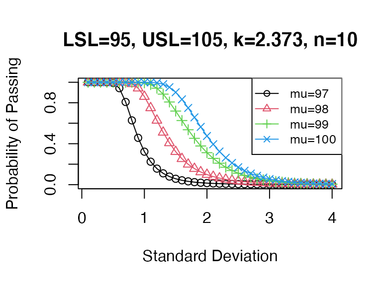
 mu <- seq(95, 105, 0.1)
 pp5 <- sapply(X=mu, FUN =  PPQ_pp, sigma=0.5, n=10, Llim=95, Ulim=105, k=2.373)
 pp6 <- sapply(X=mu, FUN =  PPQ_pp, sigma=1, n=10, Llim=95, Ulim=105, k=2.373)
 pp7 <- sapply(X=mu, FUN =  PPQ_pp, sigma=1.5, n=10, Llim=95, Ulim=105, k=2.373)
 pp8 <- sapply(X=mu, FUN =  PPQ_pp, sigma=2, n=10, Llim=95, Ulim=105, k=2.373)
 pp9 <- sapply(X=mu, FUN =  PPQ_pp, sigma=2.5, n=10, Llim=95, Ulim=105, k=2.373)
 plot(mu, pp5, xlab="Mean Value", main="LSL=95, USL=105, k=2.373, n=10",
 ylab="Probability of Passing", type="o", pch=1, col=1, lwd=1, ylim=c(0,1))
 lines(mu, pp6, type="o", pch=2, col=2)
 lines(mu, pp7, type="o", pch=3, col=3)
 lines(mu, pp8, type="o", pch=4, col=4)
 lines(mu, pp9, type="o", pch=5, col=5)
 legend("topright", legend=paste0(rep("sigma=",5),seq(0.5,2.5,0.5)), bg="white",
 col=c(1,2,3,4,5), pch=c(1,2,3,4,5), lty=1, cex=0.8)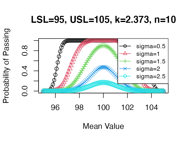
PPQ_occurve: plots OC curves for specification test and PPQ plan, with the options of customizing CQA name, unit, number of batch, optimizing the plans, etc.
PPQ_occurve(attr.name = "Sterile Concentration Assay", attr.unit="%LC", Llim=95, Ulim=105, mu=98, sigma=seq(0.1, 10, 0.1), n=10, k=2.373)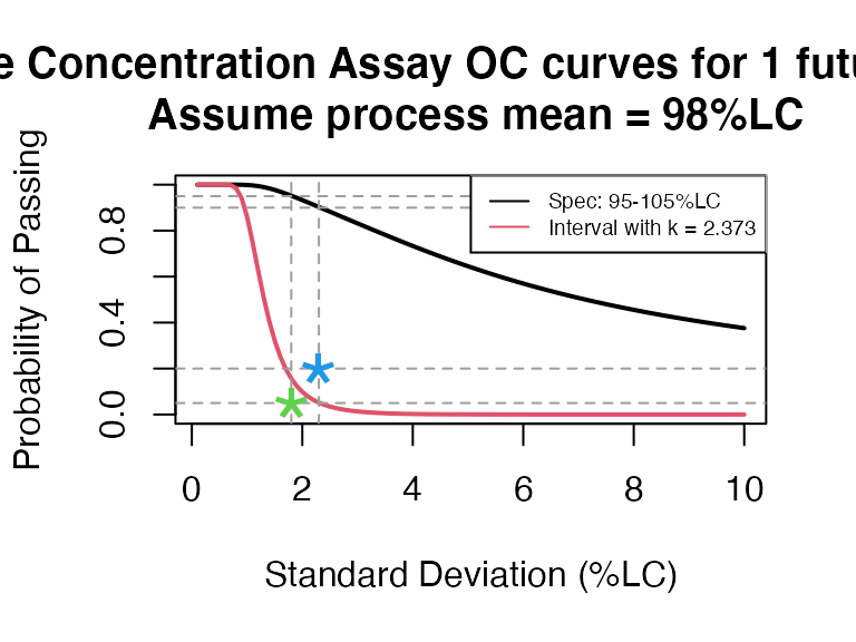
The function can also optimize the baseline and high performance sampling plan1 by using add.reference option.
PPQ_occurve(attr.name = "Sterile Concentration Assay", attr.unit="%LC", Llim=95, Ulim=105, mu=98, sigma=seq(0.1, 10, 0.1), n=10, k=2.373, add.reference=TRUE)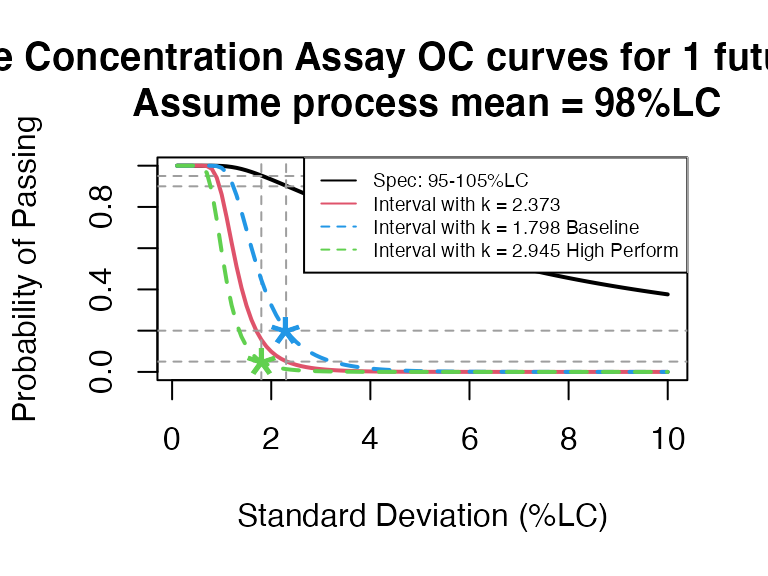
We can also optimize and show the Baseline and High performance reference lines only:
PPQ_occurve(attr.name = "Sterile Concentration Assay", attr.unit="%LC", Llim=95, Ulim=105, mu=98, sigma=seq(0.1, 10, 0.1), n=10, add.reference=TRUE)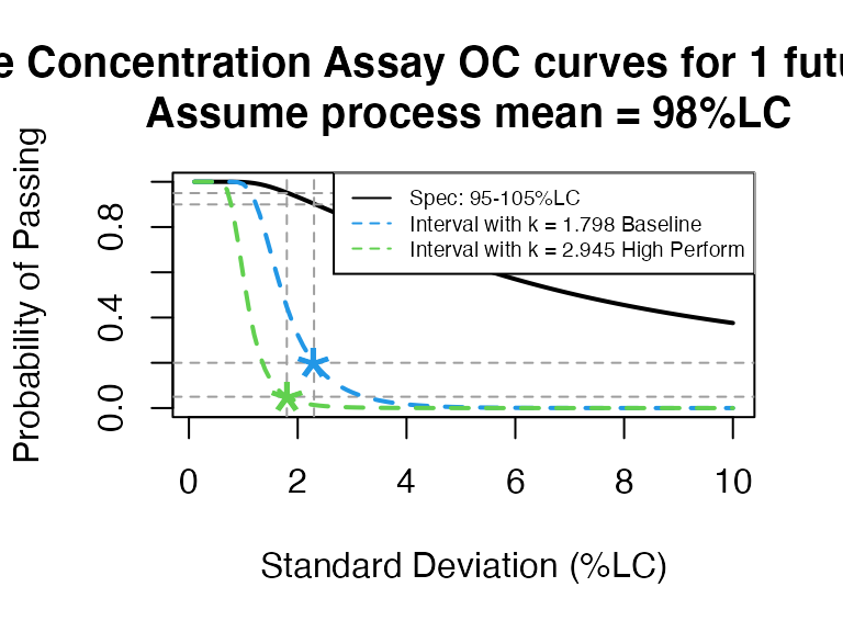
Since \(k=2.373\) is between 1.798 (baseline) and 2.945 (high performance), the 95% confidence interval is suitable for this PPQ plan.
PPQ_ctplot: Heatmap (or Contour Plot) for PPQ assessment with parameter space.
mu <- seq(95,105,0.05)
sigma <- seq(0.1,1.75,0.05)
PPQ_ctplot(attr.name = "Sterile Concentration Assay", attr.unit = "%LC", Llim=95, Ulim=105, mu = mu, sigma = sigma, k=2.373)
test <- data.frame(mu=c(97,98.3,102.5), sd=c(0.55, 1.5, 1.2))
PPQ_ctplot(attr.name = "Sterile Concentration Assay", attr.unit = "%LC", Llim=95, Ulim=105, mu = mu, sigma = sigma, k=2.373, test.point=test)
PPQ_ggplot: Dynamic Heatmap (or Contour Plot) for PPQ assessment with parameter space.
 mu <- seq(95, 105, 0.05)
 sigma <- seq(0.1,1.75,0.05)
 PPQ_ggplot(attr.name = "Sterile Concentration Assay", attr.unit = "%LC", Llim=95, Ulim=105, mu = mu, sigma = sigma, k=2.373, dynamic = FALSE)
PPQ_ggplot(attr.name = "Sterile Concentration Assay", attr.unit = "%LC", Llim=95, Ulim=105, mu = mu, sigma = sigma, k=2.373, test.point = test, dynamic = FALSE)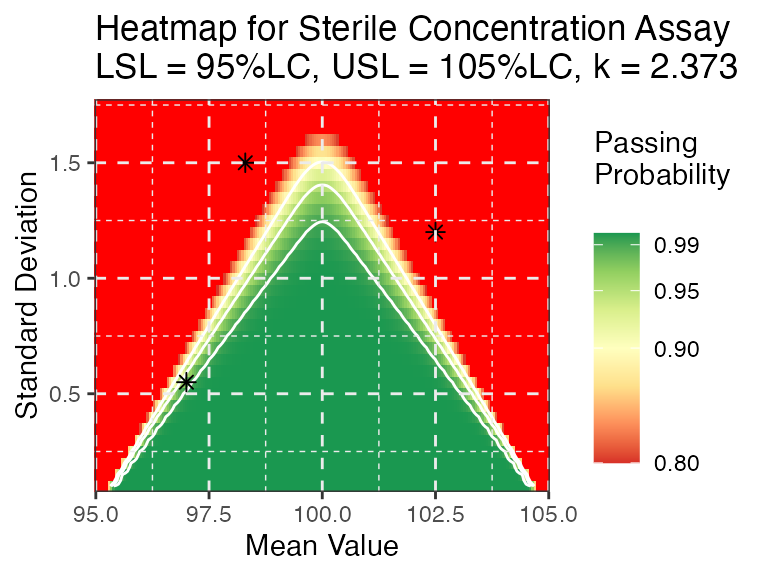
Plot a dynamic heat map. User can hover on the plot to interactively evaluate the plan with dynamic = TRUE option.
PPQ_ggplot(attr.name = "Sterile Concentration Assay", attr.unit = "%LC", Llim=95, Ulim=105, mu = mu, sigma = sigma, k=2.373, test.point = test, dynamic = TRUE)The following three functions are used for sampling plan with prediction interval.
pi_pppi_occurvepi_ctplot
pi_pp: calculates the probability of passing the PPQ test using prediction interval with confidence level \(100 \times 1-\alpha\).
Use the same example with alpha=0.05 option.
pi_pp(Llim=95, Ulim=105, mu=98, sigma=1, n=10, n.batch = 1, alpha=0.05)## [1] 0.8606111
pi_occurve: plots OC curves for specification test and PPQ plan, with the options of customizing CQA name, unit, number of batch, optimizing the plans, etc.
 pi_occurve(attr.name = "Sterile Concentration Assay", attr.unit="%LC",
 mu=97, sigma=seq(0.1, 10, 0.1), Llim=95, Ulim=105, n=10, add.reference=TRUE)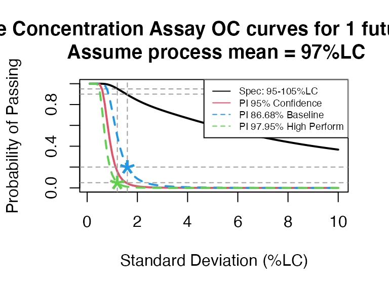
 pi_occurve(attr.name = "Sterile Concentration Assay", attr.unit="%LC",
 mu=100, sigma=seq(0.1, 10, 0.1), Llim=95, Ulim=105, n=10, add.reference=TRUE)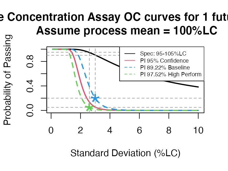
 pi_occurve(attr.name = "Sterile Concentration Assay", attr.unit="%LC",
 mu=seq(95,105,0.1), sigma=1, Llim=95, Ulim=105, n=10, add.reference=TRUE)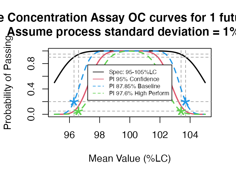

The following three functions are used for sampling plan with tolerance interval.
ti_ppti_occurveti_ctplot
ti_pp: calculates the probability of passing the PPQ test using one-sided or two-sided tolerance interval with confidence level \(100 \times 1-\alpha\).
Use the same example with alpha=0.05 option.
ti_pp(Llim=95, Ulim=105, mu=98, sigma=1, n=10, n.batch = 1, alpha=0.05, side=2)## [1] 0.9942658
ti_pp(Llim = 100, Ulim = Inf, mu=102.5, sigma=2, alpha = 0.05, coverprob = 0.675, side=1)## [1] 0.6185582
ti_occurve: plots OC curves for specification test and PPQ plan, with the options of customizing CQA name, unit, number of batch, optimizing the plans, etc.
 ti_occurve(attr.name = "Sterile Concentration Assay", attr.unit="%",
 mu=97, sigma=seq(0.1, 10, 0.1), Llim=95, Ulim=105, n=10, add.reference=TRUE)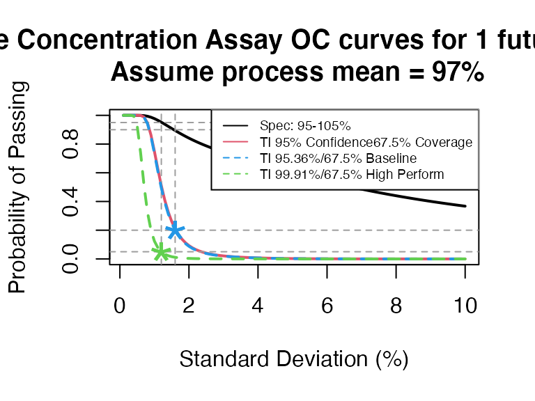
 ti_occurve(attr.name = "Sterile Concentration Assay", attr.unit="%",
 mu=100, sigma=seq(0.1, 10, 0.1), Llim=95, Ulim=105, n=10, add.reference=TRUE)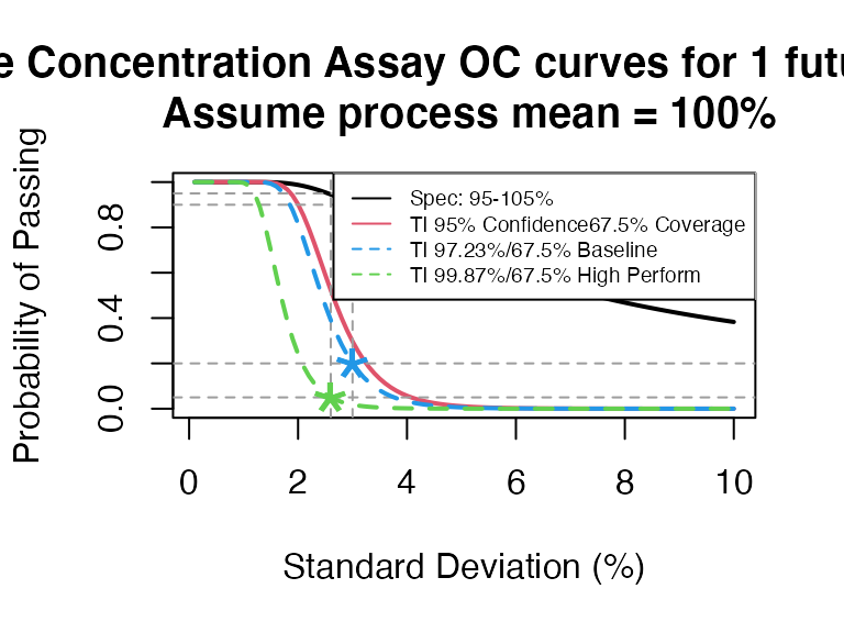
 ti_occurve(attr.name = "Sterile Concentration Assay", attr.unit="%",
 mu=seq(95,105,0.1), sigma=1, Llim=95, Ulim=105, n=10, add.reference=TRUE)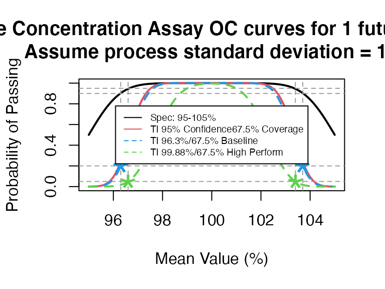
Another example is test Extractable Volume using one-sided lower tolerance interval2.
- NV = 1mL, select 5 containers and pool them together
ti_occurve(attr.name = "Extractable Volume", attr.unit = "% of NV=1mL", Llim = 100, Ulim = Inf, mu=102.5, sigma=seq(0.2, 6 ,0.05), n=40, alpha = 0.05, coverprob = 0.675, side=1, NV=1)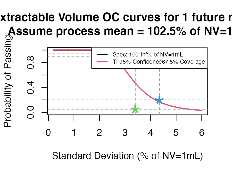
ti_occurve(attr.name = "Extractable Volume", attr.unit = "% of NV=1mL", Llim = 100, Ulim = Inf, mu=102.5, sigma=seq(0.2, 6 ,0.05), n=40, alpha = 0.05, coverprob = 0.78, side=1, NV=1)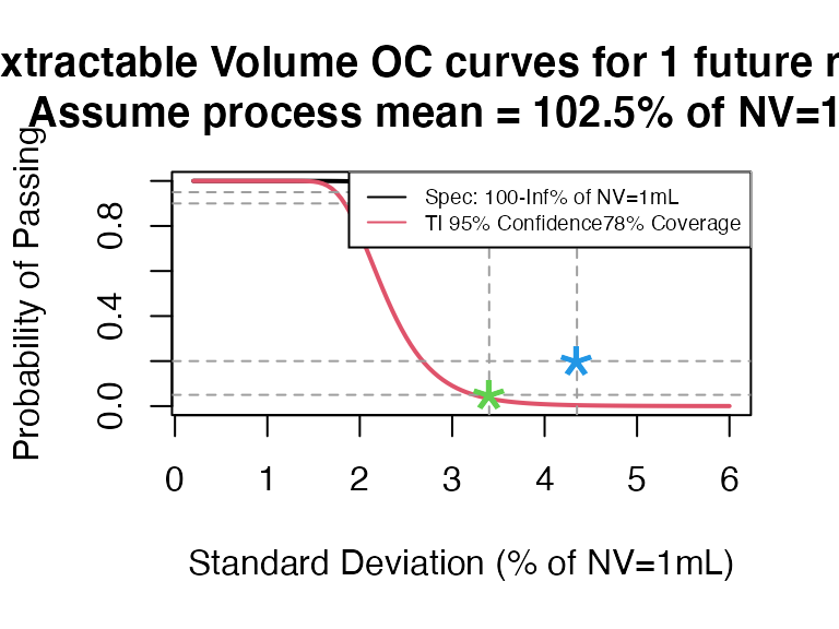
- NV = 3mL, select 5 containers but not pool
ti_occurve(attr.name = "Extractable Volume", attr.unit = "% of NV=3mL", Llim = 100, Ulim = Inf, mu=102.5, sigma=seq(0.2, 6 ,0.05), n=40, alpha = 0.05, coverprob = 0.97, side=1, NV=3)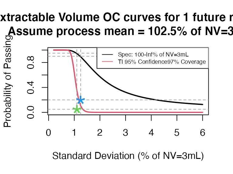
ti_occurve(attr.name = "Extractable Volume", attr.unit = "% of NV=3mL", Llim = 100, Ulim = Inf, mu=102.5, sigma=seq(0.2, 6 ,0.05), n=40, alpha = 0.05, coverprob = 0.992, side=1, NV=3)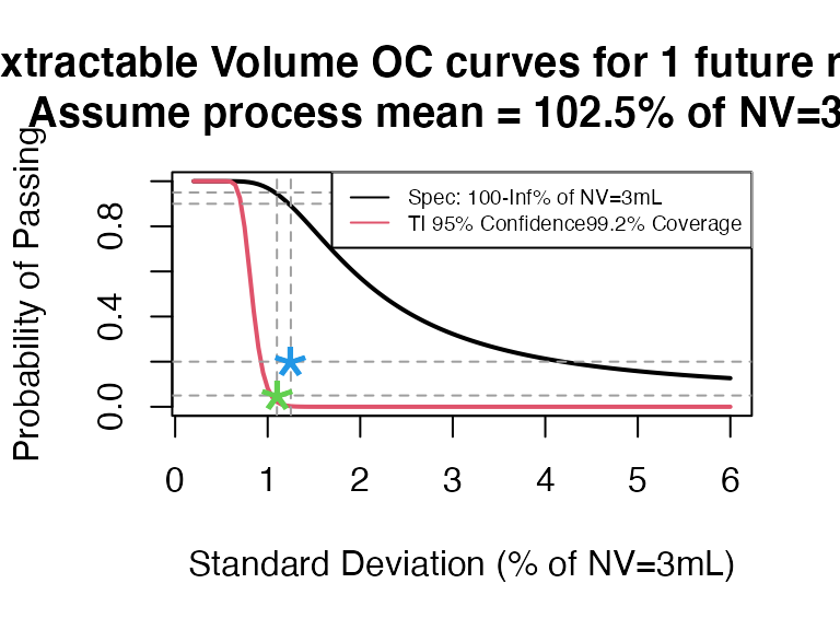
- NV = 6mL, select 3 containers but not pool
ti_occurve(attr.name = "Extractable Volume", attr.unit = "% of NV=6mL", Llim = 100, Ulim = Inf, mu=102.5, sigma=seq(0.2, 6 ,0.05), n=40, alpha = 0.05, coverprob = 0.95, side=1, NV=6)
ti_occurve(attr.name = "Extractable Volume", attr.unit = "% of NV=6mL", Llim = 100, Ulim = Inf, mu=102.5, sigma=seq(0.2, 6 ,0.05), n=40, alpha = 0.05, coverprob = 0.987, side=1, NV=6)
ti_ctplot: Heatmap (or Contour Plot) for PPQ assessment with parameter space.
mu <- seq(95, 105, 0.05)
sigma <- seq(0.1,2.5,0.05)
ti_ctplot(attr.name = "Sterile Concentration Assay", attr.unit = "%LC", Llim=95, Ulim=105, mu = mu, sigma = sigma)
Also test the Extractable Volume using one-sided tolerance interval, for example, NV = 1mL with 95% / 67.5% one-sided lower tolerance interval.
ti_ctplot(attr.name = "Extractable Volume", attr.unit = "% of NV=1mL", Llim = 100, Ulim = Inf, mu=seq(100, 110, 0.5), sigma=seq(0.2, 15 ,0.5), n=40, alpha = 0.05, coverprob = 0.675, side=1)
The package also provides two functions for a general sampling plan based on lower and/or upper specification limits.
ppheatmap_ly
pp: calculate the probability of passing general upper and/or lower specification limit.
ti_pp(Llim=-0.2, Ulim=0.2, mu=0.1, sigma=0.15, n=2)## [1] 0.02568295
heatmap_ly: plot a plain or dynamic heatmap (or contour plot) for a general sampling plan with specification limit.
heatmap_ly(attr.name = "Thickness", attr.unit = "%",Llim = -0.2, Ulim = 0.2, mu = seq(-0.2, 0.2, 0.001), sigma = seq(0,0.2, 0.001), test.point=data.frame(c(0.1,-0.05),c(0.15,0.05)), n=2, dynamic = TRUE)Burdick, R. K., LeBlond, D. J., Pfahler, L. B., Quiroz, J., Sidor, L., Vukovinsky, K., & Zhang, L. (2017). Statistical Applications for Chemistry, Manufacturing and Controls (CMC) in the Pharmaceutical Industry.↩︎
USP <1> https://www.usp.org/sites/default/files/usp/document/harmonization/gen-method/q08_pf_31_1_2005.pdf.↩︎